

A business preparing to handle a harvest may need to commit resources before it knows how much crop will arrive. A modest plan can protect its lowest result while sacrificing a large opportunity in a good season. A larger commitment can capture that opportunity and perform badly when supply disappoints. Saying that management should be cautious does not identify which comparison it should make.
On May 20, 2025, Reuters reported concern that heat and insufficient rainfall would affect the harvest in Rostov, in Russia, following spring frosts. These were assessments of an unfolding season, not the final harvest result. They provide context for examining decisions made before the relevant supply is known.
A forecast range does not choose a decision rule
The numerical exercise below is invented. It concerns commercial handling commitments, not a recommendation about planting, irrigation, insurance or investment in an actual agricultural business. Its outcomes are stipulated to make two decision rules visible. None of the amounts represents a forecast for Rostov or a reconstruction of a company's contracts.
There are three plans and three possible supply states. The plans are called small, flexible and large. These names identify rows in a comparison; they do not prove that a particular physical arrangement is flexible or cheap. Every plan must be selected before the supply state is revealed. There is no later switching option and no opportunity to buy information in this exercise.
The supply states are abundant, ordinary and poor. They are assumed to be mutually exclusive and, within this model, exhaustive: one of them occurs. Initially, no probabilities are assigned. Calling a state ordinary does not give it a greater probability. The label describes its position in the scenario set, not evidence that it is more likely than either alternative.
All results refer to the same evaluation period and the same abstract monetary unit. They are contributions after the costs included in each plan, rather than gross receipts. Continuing overhead and other excluded items are outside the exercise. Costs already included must not be deducted again. A comparison loses meaning if one plan is shown before its costs and another after them.
Write down outcomes before judging them
The small plan produces forty units in abundant supply, thirty-five in ordinary supply and thirty in poor supply. The flexible plan produces sixty-five, forty-five and twenty respectively. The large plan produces one hundred, fifty and minus ten. Those are complete scenario results under the construction, not changes relative to an unstated budget.
- Small commitment: forty, thirty-five and thirty.
- Flexible commitment: sixty-five, forty-five and twenty.
- Large commitment: one hundred, fifty and minus ten.
Read each row as one plan meeting three different possible circumstances. Read each column as three plans meeting the same circumstance. These two directions answer different questions. A row reveals the range of outcomes a committed plan could face. A column reveals which plan would have performed best if that state were the one that occurred.
No row is best everywhere. The large plan gives the highest result in abundant and ordinary supply. The small plan gives the highest result in poor supply. The flexible plan never leads a column, but that does not automatically make it irrelevant. A decision criterion can prefer a compromise that avoids a very large shortfall without maximising the result in any single state.
First check whether an alternative is dominated
A plan would be dominated if another available plan produced at least as much in every state and more in at least one, assuming no omitted difference mattered. That is not true of these rows. The flexible plan improves on the small plan in two states but performs worse in the third. The large plan similarly has gains and a downside compared with the others.
This check prevents an unnecessary debate about a plainly inferior row, but it does not choose among all remaining alternatives. Once genuine trade-offs remain, the decision-maker needs a criterion. The criterion is an expression of what is being protected or pursued. It is not another piece of weather evidence and should not be presented as if the forecast selected it.
Protecting the lowest result
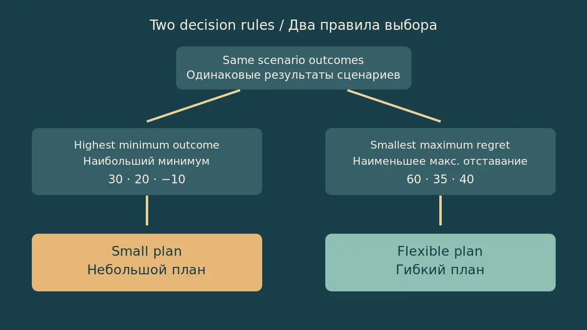
One rule looks at the worst result within each row and chooses the highest of those worst results. It is often called maximin. The small plan's floor is thirty. The flexible plan's floor is twenty. The large plan's floor is minus ten. Under this rule, the small plan is selected because thirty is the highest available floor.
The comparison does not assign a probability of one to poor supply. It asks what each plan can deliver in its least favourable listed state, then compares those floors. That distinction matters: evaluating a lower bound is not the same as forecasting that the lower bound will occur. The rule can be applied without a numerical probability distribution.
Nor does the selection establish that the small plan is safe in an unrestricted sense. Its minimum of thirty holds only across the three supplied states and under the stated outcome assumptions. An omitted disruption could produce something worse. A lower bound within a scenario table is not a guarantee against every event outside that table.
Under abundant supply, the selected small plan delivers forty while the large plan would have delivered one hundred. Maximin accepts that opportunity gap to preserve the stronger floor. This is not an arithmetic error or a hidden cost. It is the trade-off built into the rule. Someone unwilling to accept that gap may prefer a different objective, but should name the change rather than relabel the same calculation.
Measure the gap from the best plan in each state
A second comparison begins with the best achievable result in each column. In abundant supply, the benchmark is one hundred. In ordinary supply, it is fifty. In poor supply, it is thirty. These benchmarks come from plans that were available in the original comparison. They are not targets imported from a more profitable business or from an unavailable technology.
Subtract a plan's outcome from the benchmark in the same column. The resulting difference is called regret in this decision framework. It is the opportunity gap relative to the best listed plan for that state. It does not describe a manager's emotions, an additional cash payment or a penalty that a customer will charge.
For the small plan, regret is sixty in abundant supply, fifteen in ordinary supply and zero in poor supply. The calculations are one hundred minus forty, fifty minus thirty-five, and thirty minus thirty. The zero in the last column means the small plan matches the best available outcome there, not that its actual contribution is zero.
For the flexible plan, the gaps are thirty-five, five and ten. For the large plan, they are zero, zero and forty. The final forty is particularly important: the large plan produces minus ten when the best available plan would have produced thirty. The gap between those results is forty, but the large plan's actual negative contribution remains ten. Subtracting forty again would invent a second loss.
Limiting the largest opportunity gap
The minimax-regret rule takes the largest regret in each row and selects the smallest of those maxima. The small plan's maximum regret is sixty. The flexible plan's is thirty-five. The large plan's is forty. The flexible plan therefore wins this comparison, even though it is not the best plan in any individual supply state.
That result is not a compromise chosen by intuition after looking at the names. It follows directly from the specified objective. The flexible plan keeps every gap within thirty-five. The small plan permits a gap of sixty, and the large plan permits one of forty. The rule protects against being too far behind the best feasible alternative once the state is known.
The selected flexible plan still has a lower worst contribution than the small plan: twenty rather than thirty. It would be misleading to describe minimax regret as simply another way of maximising the floor. The two criteria compare different quantities. One protects an absolute result; the other limits a relative shortfall against a state-dependent benchmark.
Neither calculation needs the probabilities of the states, but neither is free of judgement. Choosing which criterion matters is itself a judgement about the objective. The table cannot prove that every organisation should value the stronger floor more than the smaller opportunity gap, or the reverse. A transparent decision records both the outcome comparison and the rule used to select a plan.
Equal weights add an assumption
A tempting response to missing probabilities is to average the three outcomes. The small plan's simple mean is thirty-five. The flexible plan's is one hundred and thirty divided by three, approximately forty-three point three. The large plan's is one hundred and forty divided by three, approximately forty-six point seven. Ranking those means selects the large plan.
This is a third answer, but not a probability-free expected-value calculation. Treating the simple mean as an expected result gives each state a probability of one third. That may be a deliberately chosen assumption; it is not established merely because three scenarios were written down. Scenario count and evidence about likelihood are different things.
The distinction becomes clear if an analyst describes abundant supply through several subcases while leaving poor supply as one case. An unweighted average of the newly expanded list would change the implicit weights. Nothing about the weather need have changed. The way the analyst organised the list would have changed the calculation instead.
An explicitly weighted analysis can be useful when its probabilities have a defensible basis or when the purpose is to test stipulated beliefs. Here, however, probabilities were intentionally not supplied. Introducing equal weights should therefore be reported as a new scenario assumption, not as a neutral way to escape uncertainty or a correction to the other two rules.
Keep the benchmark tied to feasible alternatives
Regret depends on which alternatives are available. If a comparison includes a plan that the business cannot implement, that plan might set an unreachable benchmark and inflate the apparent shortfall of the feasible choices. Availability must therefore be considered before interpreting the gap, not added as a footnote after a preferred row has been selected.
Our exercise assumes that all three plans are feasible and that their outcomes already reflect their defined commitments. It does not specify borrowing capacity, contractual permissions or physical requirements. Adding such constraints would change the decision problem. A plan with an attractive numerical result cannot be made executable by the arithmetic alone.
The same discipline applies to alternative actions within a plan. Calling the middle row flexible does not authorise management to combine its favourable results with those of another row after the state is revealed. The row is a preselected policy with fixed scenario outcomes. A genuine switching option would require a different description and its own consequences.
Scenario coverage matters more than reassuring labels
The poor-supply state is the least favourable state for every plan in the original table. But a reader should not assume that the word poor captures every commercial difficulty. A scenario could omit disruption to handling, changes in realised prices or another condition that matters to the defined result. The model has no information from which to quantify those possibilities.
A useful review asks whether the states cover the uncertainty relevant to the decision and whether the outcomes are internally consistent. It should not silently add every imaginable danger to one row while leaving the others unchanged. Comparable plans must face comparable scenario definitions. Otherwise apparent caution could come from an uneven construction rather than a genuine difference between commitments.
It is also possible for all three plans to perform badly in a newly considered state. A relative regret measure might remain small because every feasible alternative is similarly weak. That would not make the absolute loss acceptable. Looking at the underlying outcome table alongside the regret table prevents a small relative gap from concealing a poor result.
A result and its comparison need separate names
For each selected plan, report the actual scenario contribution and, separately, the gap from the best alternative. The small plan in abundant supply contributes forty and has regret of sixty. The large plan in poor supply contributes minus ten and has regret of forty. Combining those statements into a single figure would obscure what the business receives and what the analyst is comparing.
Likewise, avoid describing the maximum regret as an expected loss. A maximum identifies the largest gap in the supplied set. An expectation requires probabilities. Both can be meaningful, but one cannot be substituted for the other by changing the heading above a spreadsheet column. The labels are part of the analysis, not decoration added after the numbers are finished.
Do not let hindsight rewrite the original objective
After abundant supply occurs, the large plan will look best in this table. That does not establish that management knew the state in advance. A decision taken under uncertainty should be assessed against the information and objective available when it was made. Otherwise every realised state would retrospectively demand its own winning plan, an impossible instruction for an earlier one-time commitment.
Conversely, naming a criterion does not excuse a badly constructed comparison. Incorrect outcomes, omitted feasible alternatives or an objective that does not match the organisation's needs remain substantive problems. The value of documenting the rule is that those questions can be examined separately from whether one particular season happened to reward the selected plan.
- State which commitments must be chosen before supply becomes known.
- Use one period and one net-result definition across all plans.
- Separate scenario assumptions from evidence about probabilities.
- Calculate column benchmarks only from feasible alternatives.
- Keep actual contributions distinct from opportunity gaps.
- Record the decision criterion before reviewing the realised outcome.
Different protections produce different choices
The invented table yields three distinct selections. Protecting the highest minimum contribution chooses the small plan. Limiting the largest gap from the state-specific best plan chooses the flexible plan. Adding equal probabilities and comparing means chooses the large plan. The disagreement is informative: it reveals different objectives or assumptions, not three competing arithmetic answers to an identical question.
A forecast can describe uncertainty without resolving those objectives. Before treating a plan as prudent, identify what it protects: a floor, an opportunity gap or an expected result under stated probabilities. Keeping those ideas separate makes the commercial discussion more precise and prevents a favourable scenario, a worst case or an average from quietly standing in for all the others.