
An advertising campaign can receive credit for many orders without adding enough business to cover its own expense. The difficult number is not the number of purchases recorded after an advertisement. It is the difference between the purchases made with the campaign and the purchases that would have occurred under a specified alternative. A randomised comparison can help estimate that difference, but it does not turn every purchase into an individually identifiable advertising success.
On February 25, 2026, Kommersant reported Kokoc Performance's estimate that the 2025 performance-marketing market in Russia reached RUB 450 billion. Contextual advertising, targeted advertising and retail media were the largest categories. This was a named market participant's estimate, not an official measurement of additional sales caused by advertising.
The size of spending makes a narrower buyer-side question worth examining: what evidence connects a campaign expense to additional contribution? The fictional experiment below answers that question under explicit assumptions. It is not a study of the companies in the news report, a claim about typical advertising performance or a reconstruction of any marketplace's customers.
Decide what the experiment is comparing
Imagine an anonymous seller with two thousand eligible people. Before the campaign starts, a random procedure assigns one thousand to a treatment group and one thousand to a control group. The campaign is made available to the treatment group and withheld from the control group. All other commercial conditions are held the same in this simplified example. Both groups face the same product, price and purchase window.
The comparison concerns assignment to this campaign, not a comparison between people who chose to click and people who did not. Clicking is a behaviour that may itself reveal unusually strong buying intent. Selecting clickers after the campaign starts would change the question and surrender the clean assignment mechanism. A customer who never clicks remains in the group to which that customer was originally assigned.
The experiment also needs a defined alternative. Here the control group receives ordinary business activity without the particular campaign being tested. It does not live in a world without advertising, recommendations, existing brand knowledge or other reasons to buy. The estimate therefore concerns adding this one intervention to the specified background. It cannot automatically be described as the value of all the seller's marketing.
Google's Conversion Lift documentation describes comparing exposed and withheld groups to measure additional conversions. That supplies a methodological reference, not evidence about the fictional seller. It is not a claim about the service's availability in a particular country or a recommendation to use a particular platform.
Keep assignment separate from subsequent behaviour
Random assignment is useful because the groups are formed before the response being measured. It prevents the analyst from deliberately putting enthusiastic buyers in one group and reluctant buyers in the other. It does not promise that the two realised groups will contain exactly the same mix of every characteristic. Chance differences remain possible, especially when the outcome is variable or the experiment is small.
For the model, assume assignment is implemented correctly, all purchases are observed consistently and customers do not pass the treatment to the control group. There are no simultaneous price changes, special product allocations or other interventions that differ between the groups. These are simplifying conditions of the example, not assertions that commercial experiments satisfy them automatically.
The unit of assignment and the unit of measurement must stay visible. We assign people and count their orders during one common window. A person might place more than one order; the model does not need to equate buyers with transactions. What matters is that the same counting rule applies in both groups and that no one is removed simply because the outcome looks inconvenient.
A missing purchase record is not the same as no purchase. If treatment purchases are easier to observe than control purchases, an apparent difference can partly reflect measurement. Likewise, comparing a completed treatment week with an incomplete control week would manufacture a difference in exposure to time. The experiment requires a common observation boundary before any contribution calculation begins.
Two order totals produce a point estimate
At the end of the fictional observation period, the treatment group has placed 150 orders and the control group 100. Because the groups have equal assigned sizes, the simple difference is fifty orders. That is the model's point estimate of the campaign's incremental orders in the treatment arm. It is not a list of fifty transactions that can be individually marked as caused by the campaign.
Separately, the seller's attribution system credits 120 treatment-group orders to the campaign under its chosen reporting rule. The remaining thirty treatment orders are not credited under that rule. These numbers describe a classification of observed transactions. They do not supply the unobserved alternative outcome for each purchaser, and they do not change the treatment group's total of 150.
The contrast between 120 credited orders and an estimated fifty additional orders is not proof that the attribution system counted seventy nonexistent purchases. All 120 credited orders may be real. The two calculations answer different questions: one assigns reporting credit to transactions; the other estimates a difference against a withheld comparison group. Calling the gap fraud would go beyond the evidence.
It is equally incorrect to identify the thirty uncredited orders as the complete baseline. The control group suggests a larger level of ordinary purchasing under the defined alternative, subject to uncertainty. A reporting label cannot reveal which particular treatment customer would have bought anyway. The experiment estimates an aggregate effect without recovering every person's missing alternative history.

Turn the estimated increment into contribution
Now give the fictional orders a simple economic structure. Every order earns ten money units of revenue and leaves four units after the avoidable order-level costs included in the model. The campaign costs 300 units. Prices, order sizes and the four-unit contribution are deliberately identical across the comparison, so the arithmetic does not conceal a product-mix or discounting effect.
The attribution report associates 120 orders with 1,200 revenue units. Dividing that revenue by the 300-unit campaign expense gives an attributed revenue return of four. This ratio is a revenue measure, not a profit measure. Even before considering the experimental comparison, it would be wrong to treat every revenue unit as money available to cover advertising expense.
Using the experimental point estimate instead gives fifty additional orders and 500 additional revenue units. The incremental revenue-to-spend ratio is 500 divided by 300, or five thirds. More importantly for this specific decision, the estimated additional order contribution is fifty multiplied by four, or 200. After subtracting the 300-unit campaign expense, the estimated incremental contribution is minus 100.
The result is not the seller's net profit. It leaves out the wider business, fixed overhead, tax, financing and other items outside the defined comparison. Nor does it prove that this campaign has a negative true effect on contribution: the order difference is an estimate. It shows what economic conclusion follows when that particular point estimate is combined with the stipulated contribution and expense.
The same calculation can be checked without a ratio
The treatment group's 150 orders produce 600 units of contribution before campaign expense. Subtracting 300 leaves 300. The control group's 100 orders produce 400 units without that expense. Comparing these two totals gives 300 minus 400, again minus 100. This direct check helps prevent a revenue multiple from displacing the underlying comparison.
Only expenses caused by the defined treatment belong in this incremental calculation. The example stipulates that the 300 units are such an expense. If a real contract bundled other activities or if the two groups had different order-level costs, the analyst would need a different specification. Quietly importing those complications after seeing the result would make the model less transparent, not more realistic.
A break-even count is not a confidence threshold
At four units of contribution per additional order, the campaign needs seventy-five additional orders to cover its 300-unit expense. That is an economic threshold within the fictional model. It does not mean seventy-five attributed orders are sufficient, and it does not define a statistical test. The current point estimate of fifty falls twenty-five orders below that economic threshold.
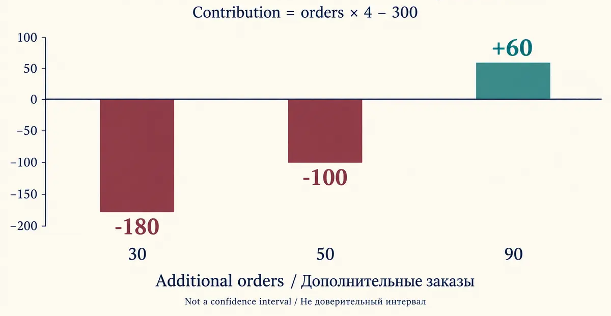
To see the sensitivity, suppose the relevant incremental-order estimate were thirty, fifty or ninety while the other assumptions remained fixed. Those cases yield 120, 200 or 360 units of order contribution. After campaign expense, the corresponding figures are minus 180, minus 100 and plus sixty. The three cases deliberately show how uncertainty about additional orders can matter to the decision.
These are scenarios, not a confidence interval. They have no assigned probabilities and were not calculated from the distribution of experimental outcomes. Presenting them as a statistical range would give a simple arithmetic exercise authority it has not earned. A proper uncertainty assessment would require the actual experiment's design and outcome data, not merely three convenient numbers.
The economic threshold and statistical uncertainty should therefore remain on separate lines of a decision record. One asks how much additional business is needed under the specified economics. The other asks what the evidence supports about the unknown effect. A point estimate above a threshold can still be imprecise; a precise estimate can still fall below the contribution needed to justify the expense.
Protect the comparison when the campaign meets reality
A control group can be contaminated when people receive the campaign through another route or share an offer across the assignment boundary. The problem is not merely untidy reporting. It changes the contrast that the experiment actually creates. If both groups receive much of the intervention, the intended campaign-versus-withheld comparison may no longer describe what happened.
Changes in the treatment can create a similar difficulty. If the advertised product runs out only for one group, the observed difference includes that availability difference. If an additional discount accompanies the campaign, the experiment tests the combined package rather than advertising alone. Those may be legitimate business questions, but the conclusion must name the package that was actually assigned.
The observation period is another boundary, not a clerical detail. Purchases before assignment cannot be outcomes of the assigned intervention. Purchases after the chosen closing date are outside this model. A longer-term effect might matter, but it cannot be inserted as a favourable number without evidence. The present example deliberately makes no lifetime-value or enduring brand-effect claim.
Finally, the tested audience limits the interpretation. These two groups represent the eligible people in the fictional experiment. Multiplying the estimated effect by every customer the seller has ever served would add an untested assumption about transferability. Different audiences, campaign intensity and commercial conditions can require their own evidence rather than a mechanical scale-up of fifty orders.
Record the decision in the order the evidence supports
There is also a distinction between learning from the completed test and promising the same result from a subsequent campaign. Even an impeccably implemented comparison describes an intervention at a particular scale. A larger budget might reach different people or expose the same people more often. Neither change is represented by the fixed groups and fixed expense in this example. A decision to expand would therefore introduce a new question rather than merely repeat the subtraction.
Recording that boundary need not make the analysis indecisive. The team can state precisely that the completed comparison produced an estimated fifty additional orders and minus 100 incremental contribution under the stated economics, while reserving judgment about a redesigned intervention. That is more informative than either declaring all advertising unsuccessful or asserting that a high attributed revenue multiple settles the case. The experiment has a useful answer because its question is bounded.
A useful decision record starts with assignment and ends with economics. Reversing that order encourages the team to search for a flattering measure after seeing whether the campaign appears successful. The following questions keep the fictional example's logic intact without turning it into a platform-specific implementation guide.
- What exactly was assigned, to whom, and what activity remained available to the control group?
- Were all assigned participants retained under a common outcome definition and observation window?
- Which number is an attribution total, and which is an experimental point estimate?
- What uncertainty accompanies that estimate, separately from any illustrative scenarios?
- Which contribution per additional order and which treatment expense belong to the economic comparison?
- Does the conclusion stop at the tested audience, intervention and period?
The model does not show that performance advertising is ineffective. It shows why a campaign credited with 120 real orders and a revenue multiple of four can still have a negative estimated incremental contribution under stated assumptions. The missing step is neither a new dashboard label nor a larger collection of clicks. It is a defensible comparison against a defined alternative, followed by an economic calculation that respects the uncertainty of that comparison.