

An order for one product can create a selling problem for another when both emerge from the same production batch. The customer may want more of the first output without wanting any of the second. A processor therefore needs to evaluate the bundle it will actually produce, not just the order that attracted its attention. Strong demand on one side can improve the opportunity without settling the economics of the whole batch.
On July 11, 2025, Reuters reported that USDA had raised its forecast for soybean-oil use in biofuels in the United States for the 2025/26 marketing year. That was an outlook, not evidence of subsequently realised consumption. It provides a dated starting point for examining the economics of joint outputs.
A July 1, 2025 USDA Economic Research Service explanation describes crushing as extracting meal and oil from soybeans and links processing investment to demand for both. That earlier page supplies process context, not confirmation of the later revised forecast. It provides no basis for the fictional yields used below.
A joint output is not a product chosen independently
There is an important difference between choosing a production mix and selling joint outputs. In a flexible product-mix problem, a business might devote a machine's time to one item rather than another. In the deliberately fixed process considered here, another batch produces both outputs together. Choosing the additional batch is therefore different from choosing twenty units of the first output alone.
This difference changes the commercial question. An attractive order has to be considered alongside the receipts available from the accompanying product. Calling that second product incidental does not remove it from the calculation. Nor does assigning it a small share of the accounting cost create a buyer. The physical bundle and the available sales opportunities remain the starting point.
The following model is an abstract two-output processor, not a reconstruction of a soybean plant. Its labels A and B represent separate saleable outputs. They are not technical grades or measured oil and meal yields. Fixing the bundle makes one business mechanism visible: the decision to run an additional batch depends on what can be realised from both products, after the costs that the decision would cause.
Define one batch in physical and monetary units
Suppose one additional batch consumes one hundred physical units of input and produces twenty units of A and eighty units of B. The example assumes no physical loss and no ability to change that split. Those are simplifying assumptions, not engineering claims. Every output unit is sold immediately through a specified outlet; there is no inventory build, storage delay or later speculative sale.
The avoidable input and processing cost of that batch is ninety accounting units. This means the cost is incurred if the batch is undertaken and avoided if it is not. Fixed overhead, tax, financing and the cost of installed capital are outside the calculation. Revenue minus ninety is therefore an incremental contribution under these assumptions, not the plant's net profit.
Keep the two kinds of units separate. One hundred describes physical input. Ninety describes expenditure. Adding them would have no meaning. Likewise, twenty units of A do not create forty of revenue until a stipulated selling value of two per unit is applied. Preserving quantity, value per unit and total receipt in separate columns makes the model easier to check.
The unconstrained outlet case
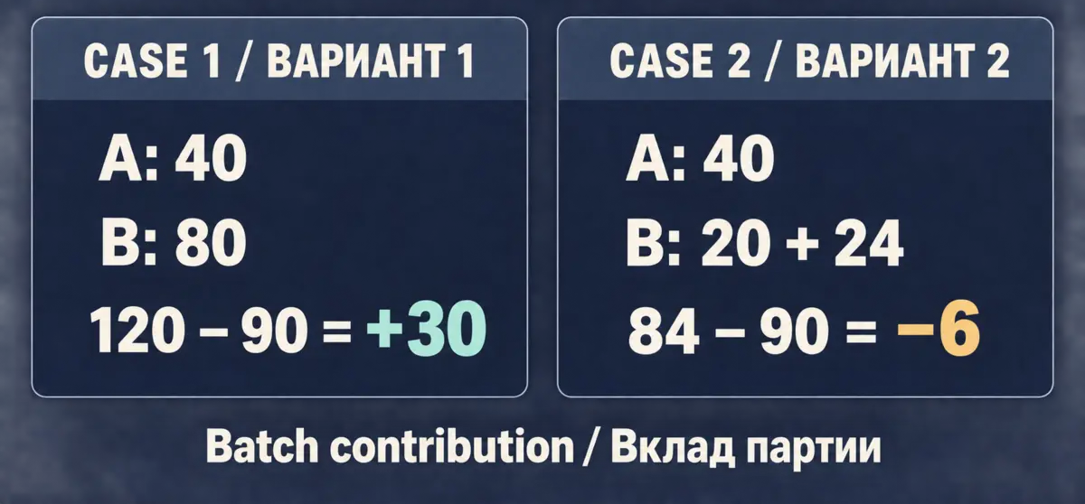
In the first case, all twenty A units sell for two each, producing forty. All eighty B units sell for one each, producing eighty. Combined revenue is one hundred and twenty. Subtract the avoidable cost of ninety and the batch contributes thirty. That positive amount exists at the level of the entire bundle; no allocation of shared cost between A and B is needed to calculate it.
It would still be wrong to report thirty as total business profit. The model has not asked whether the plant covers its continuing overhead or earns a return on its past investment. The narrower result is that undertaking this additional batch adds thirty before those excluded items, given the stated receipts and avoidable expenditure.
The same order can accompany a weaker second outlet
Now leave the A order unchanged. It still takes twenty units at two each, so the receipt remains forty. Change only the outlets available for the new batch's B output. One outlet accepts twenty units at one each. A separate outlet accepts the remaining sixty at a net realisation of four tenths per unit. These prices and quantities are stipulated, external to the model and available immediately.
The first B outlet produces twenty. The second produces twenty-four. Total revenue from B is forty-four, and total revenue from the batch is eighty-four. Against the same avoidable cost of ninety, the incremental contribution is minus six. Every physical unit has been sold. The negative contribution does not arise from unsold stock or slow collection; it arises from the receipts available for the bundle.
This is not a claim that an actual processor faces those outlets or that new production necessarily pushes down market prices. No price response is modelled. Nor are any existing sales repriced. The exercise simply compares two sets of commercial opportunities for one new batch. The attractive A order is identical in both, but the complete batch result changes from plus thirty to minus six.
Calculate the remaining receipt rather than guessing it
The second case can be turned into a useful threshold calculation. The A order contributes forty of revenue and the first B outlet another twenty. Together they provide sixty. To cover the ninety of avoidable expenditure, the remaining sixty B units must bring in thirty. Their required net realisation is therefore half an accounting unit each.
At four tenths, those units produce twenty-four and the batch falls six short. At half a unit, they produce thirty and the incremental contribution is zero. At six tenths, they produce thirty-six and the contribution is plus six. These are exact results of the invented inputs, not a soybean market break-even estimate or a forecast of any future product quotation.
The threshold also has a limited meaning. Zero incremental contribution here means that the additional batch covers the expenditure that was defined as avoidable. It does not mean the business is viable overall or that running at this level finances renewal of the plant. A calculation about one additional action cannot silently answer a question about all the costs of ownership.
Shared-cost allocation does not change the batch receipt
A product report may divide the common ninety of expenditure between A and B. That can help organise accounting, but it must not be confused with changing the cash consequences of the additional batch. In the weak-outlet case, total receipts remain eighty-four regardless of the allocation. The batch's incremental contribution remains minus six.
For example, assign thirty of shared cost to A and sixty to B. Against receipts of forty and forty-four, the displayed product differences are plus ten and minus sixteen. Alternatively, assign fifty to A and forty to B. The displayed differences become minus ten and plus four. In both versions, adding the two differences gives minus six. Only the appearance of the product columns has changed.
These allocations are invented arithmetic examples, not recommendations about financial reporting standards. Their purpose is to expose an analytical trap. A manager looking only at the positive A column in the first version could describe an attractive product while overlooking the complete batch. A manager looking only at the positive B column in the second version could make the opposite mistake with the same underlying receipts.
Once outputs are physically linked in the model, a favourable allocated margin cannot justify assuming that only the favourable product will be produced. The decision still concerns the bundle. If a different production method or external purchase could supply A alone, that would be another alternative requiring its own evidence and calculation, not a feature already present in this one.
Existing business and the next batch are separate comparisons
A plant might have established outlets for earlier production while facing different opportunities for additional units. Applying an average receipt from the existing book to the new batch would assume that those terms extend to it. That assumption could be right or wrong, but it needs to be stated. A historical average does not create additional demand at the same value.
Conversely, the weaker outlets for a new batch should not automatically be applied to all previous sales. Our model does not reopen existing contracts or change completed transactions. Its scope is the incremental bundle. Expanding that scope without evidence would turn a small decision model into an unsupported estimate of the processor's overall earnings.
The useful comparison names its boundary explicitly: which batch, which outlets, which receipts and which costs change if the action is taken? Continuing costs may matter greatly to the business without changing in this particular comparison. Leaving them outside the incremental calculation is not declaring them unimportant. It is preserving the question that the calculation was designed to answer.
A sales plan must represent both outputs
For the fictional processor, a complete commercial plan would connect each output quantity with the outlet assumed to take it. The most prominent order would occupy only part of that plan. The remainder would show whether another buyer exists for the accompanying output and what net realisation has been used. This is a statement of model inputs, not a claim about undisclosed industry contracts.
- Record the physical output bundle associated with one additional batch.
- Separate the receipt for the main order from receipts for every accompanying saleable output.
- Identify which outlet quantities apply to additional units rather than existing commitments.
- Use a consistent net-receipt basis so that selling costs are not counted twice or omitted.
- Compare the complete receipt with the expenditure caused by undertaking that batch.
In this exercise, the lower outlet value is already net. Subtracting an invented extra selling charge from it would change the assumptions and might count a cost twice. Equally, using a gross price in one column and a net price in another would make the comparison inconsistent. The model does not need many digits; it needs the same definition on both sides.
Quantities must also be assigned only once. If the first B outlet takes twenty, the second takes sixty, not eighty. The physical check gives twenty A plus eighty B, matching the stipulated one hundred output units. The monetary check gives forty plus twenty plus twenty-four, or eighty-four. These totals need not equal each other because one measures goods and the other receipts.
Check separately that the ninety of batch cost is deducted only once. Subtracting the full amount from each product and then adding the results would understate contribution. If cost is allocated, the allocations must sum to ninety. These checks preserve the same result across different table layouts and let another reader reproduce the calculation without relying on a verbal explanation of which column was intended to represent what.
Sensitivity belongs to a specific input
The half-unit threshold makes the importance of the residual outlet visible, but it is not the only input that could change in another scenario. A different A receipt or a different avoidable batch cost would move the required amount. An explicit sensitivity exercise changes one stipulated input, holds the others fixed and recalculates the bundle. It does not assert that the market will make that change.
For instance, an additional six of revenue from A would offset the six-unit shortfall in the weak-outlet case, all else equal. A six-unit reduction in avoidable cost would do the same. Those arithmetic equivalences do not prove that either improvement is commercially available. They identify the size of a difference, not a route to obtaining it.
That distinction keeps the analysis practical. It can show what would have to change before the result changes sign without claiming that management can control every input. Joint production links quantities; it does not guarantee favourable buyers, values or costs. A sound discussion separates the physical relationship from the commercial assumptions placed around it.
The decision follows the bundle
The central lesson is not that demand for the first product is unimportant. It is that this demand is incomplete evidence for a decision that creates two products together. The fictional order for A remains attractive in isolation while the available receipts for B determine whether the complete additional batch contributes thirty or loses six before excluded costs.
Following the bundle avoids two shortcuts: treating an order for one output as a sale of the whole batch, and treating an allocated product margin as the result of the physical decision. Quantities, outlets and avoidable expenditure must meet in the same calculation. Only then can the processor describe what another batch would add under the stated conditions.